A Python Guide to the Fibonacci Sequence

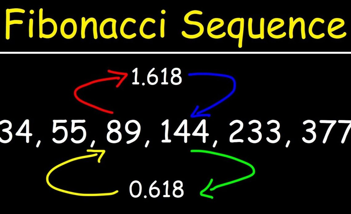
The Fibonacci sequence is a pretty famous sequence of integer numbers. The sequence comes up naturally in many problems and has a nice recursive definition. Learning how to generate it is an essential step in the pragmatic programmer’s journey toward mastering recursion. In this tutorial, you’ll focus on learning what the Fibonacci sequence is and how to generate it using Python.

In this tutorial, you’ll learn how to:

• Generate the Fibonacci sequence using a recursive algorithm
• Optimize the recursive Fibonacci algorithm using memoization
• Generate the Fibonacci sequence using an iterative algorithm

Getting Started With the Fibonacci Sequence

Leonardo Fibonacci was an Italian mathematician who was able to quickly produce an answer to this question asked by Emperor Frederick II of Swabia: “How many pairs of rabbits are obtained in a year, excluding cases of death, supposing that each couple gives birth to another couple every month and that the youngest couples are able to reproduce already at the second month of life?”

The answer was the following sequence:

The pattern begins after the first two numbers, 0 and 1, where each number in the sequence is always the sum of the two numbers before it. Indian mathematicians had known about this sequence since the sixth century, and Fibonacci leveraged it to calculate the growth of rabbit populations.

F(n) is used to indicate the number of pairs of rabbits present in month n, so the sequence can be expressed like this:

In mathematical terminology, you’d call this a recurrence relation, meaning that each term of the sequence (beyond 0 and 1) is a function of the preceding terms.

There’s also a version of the sequence where the first two numbers are both 1, like so:

In this alternative version, F(0) is still implicitly 0, but you start from F(1) and F(2) instead. The algorithm remains the same because you’re always summing the previous two numbers to get the next number in the sequence.

For the purposes of this tutorial, you’ll use the version of the sequence that starts with 0.

Examining the Recursion Behind the Fibonacci Sequence

Generating the Fibonacci sequence is a classic recursive problem. Recursion is when a function refers to itself to break down the problem it’s trying to solve. In every function call, the problem becomes smaller until it reaches a base case, after which it will then return the result to each intermediate caller until it returns the final result back to the original caller.

If you wanted to calculate the F(5) Fibonacci number, you’d need to calculate its predecessors, F(4) and F(3), first. And in order to calculate F(4) and F(3), you would need to calculate their predecessors. The breakdown of F(5) into smaller subproblems would look like this:

Each time the Fibonacci function is called, it gets broken down into two smaller subproblems because that’s how you defined the recurrence relation. When it reaches the base case of either F(0) or F(1), it can finally return a result back to its caller.

In order to calculate the fifth number in the Fibonacci sequence, you solve smaller but identical problems until you reach the base cases, where you can start returning a result:

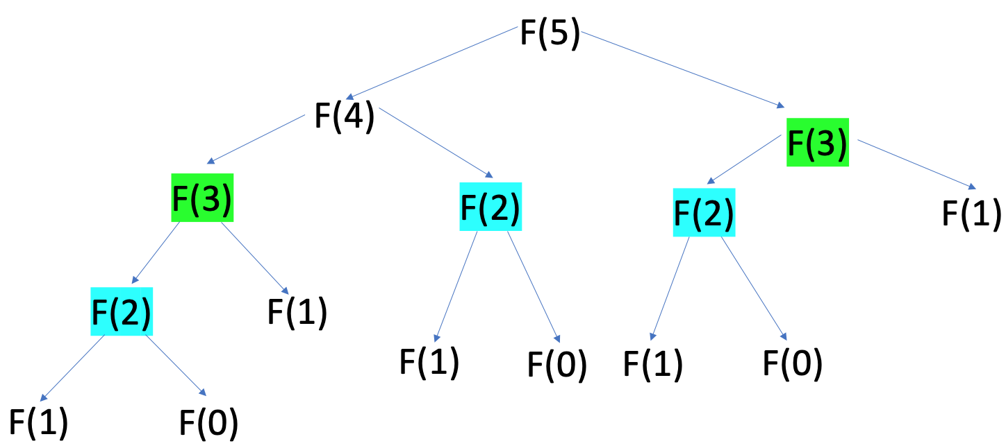
The colored subproblems on this diagram represent repetitive solutions to the same problem. If you go further up the tree, you’ll find more of these repetitive solutions. This means that to generate a Fibonacci sequence recursively, you have to calculate many intermediate numbers over and over. This is one of the fundamental issues in the recursive approach to the Fibonacci sequence.

Generating the Fibonacci Sequence Recursively in Python

The most common and minimal algorithm to generate the Fibonacci sequence requires you to code a recursive function that calls itself as many times as needed until it computes the desired Fibonacci number:>>>

>>> def fibonacci_of(n):
...     if n in {0, 1}:  # Base case
...         return n
...     return fibonacci_of(n - 1) + fibonacci_of(n - 2)  # Recursive case
...

>>> [fibonacci_of(n) for n in range(15)]
[0, 1, 1, 2, 3, 5, 8, 13, 21, 34, 55, 89, 144, 233, 377]

Inside fibonacci_of(), you first check the base case. You then return the sum of the values that results from calling the function with the two preceding values of n. The list comprehension at the end of the example generates a Fibonacci sequence with the first fifteen numbers.

This function quickly falls into the repetition issue you saw in the above section. The computation gets more and more expensive as gets bigger. The required time grows exponentially because the function calculates many identical subproblems over and over again.

To calculate F(5), fibonacci_of() has to call itself fifteen times. To calculate F(n), the maximum depth of the call tree is n, and since each function call produces two additional function calls, the time complexity of this recursive function is O(2ⁿ).

Most of those calls are redundant because you’ve already calculated their results. F(3) appears twice, and F(2) appears three times. F(1) and F(0) are base cases, so it’s fine to call them multiple times. You may want to avoid this wasteful repetition, which is the topic of the following sections.

Optimizing the Recursive Algorithm for the Fibonacci Sequence

There are at least two techniques you can use to make the algorithm to generate the Fibonacci sequence more efficient—in other words, to make it take less time to compute. These techniques ensure that you don’t keep computing the same values over and over again, which is what made the original algorithm so inefficient. They’re called memoization and iteration.

Memoizing the Recursive Algorithm

As you saw in the code above, the Fibonacci function calls itself several times with the same input. Instead of a new call every time, you can store the results of previous calls in something like a memory cache. You can use a Python list to store the results of previous computations. This technique is called memoization.

Memoization speeds up the execution of expensive recursive functions by storing previously calculated results in a cache. This way, when the same input occurs again, the function just has to look up the corresponding result and return it without having to run the computation again. You can refer to these results as cached or memoized:

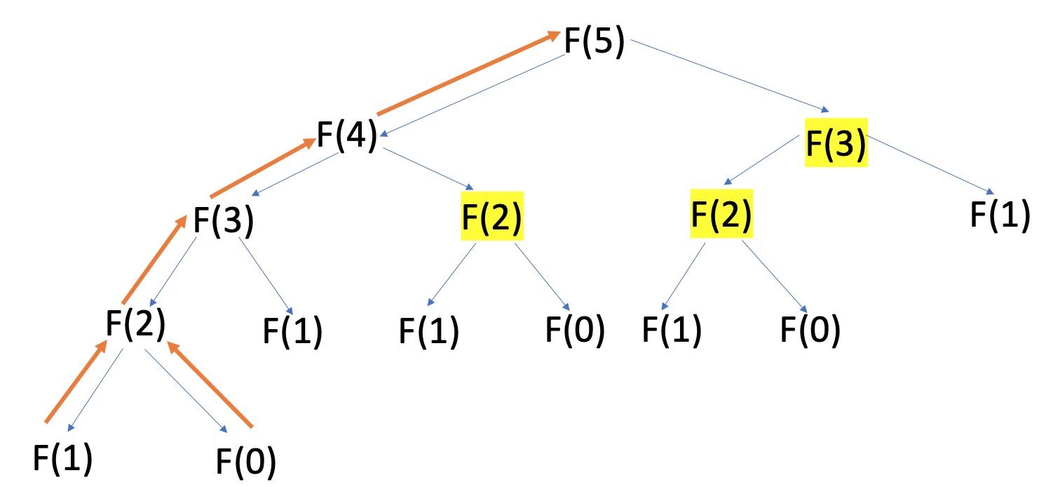
With memoization, you just have to traverse up the call tree of depth n once after returning from the base case, as you retrieve all the previously calculated values highlighted in yellow, F(2) and F(3), from the cache earlier.

The orange path shows that no input to the Fibonacci function is called more than once. This significantly reduces the time complexity of the algorithm from exponential O(2ⁿ) to linear O(n).

Even for the base cases, you can replace calling F(0) and F(1) with just retrieving the values directly from the cache at indices 0 and 1, so you end up calling the function just six times instead of fifteen!

Here’s a possible translation of this optimization into Python code:>>>

>>> cache = {0: 0, 1: 1}

>>> def fibonacci_of(n):
...     if n in cache:  # Base case
...         return cache[n]
...     # Compute and cache the Fibonacci number
...     cache[n] = fibonacci_of(n - 1) + fibonacci_of(n - 2)  # Recursive case
...     return cache[n]

>>> [fibonacci_of(n) for n in range(15)]
[0, 1, 1, 2, 3, 5, 8, 13, 21, 34, 55, 89, 144, 233, 377]

In this example, you use a Python dictionary to cache the computed Fibonacci numbers. Initially, cache contains the starting values of the Fibonacci sequence, 0 and 1. Inside the function, you first check if the Fibonacci number for the current input value of n is already in cache. If so, then you return the number at hand.

If there is no Fibonacci number for the current value of n, then you compute it by calling fibonacci_of() recursively and updating cache. The final step is to return the requested Fibonacci number.

Exploring an Iterative Algorithm

What if you don’t even have to call the recursive Fibonacci function at all? You can actually use an iterative algorithm to compute the number at position n in the Fibonacci sequence.

You know that the first two numbers in the sequence are 0 and 1 and that each subsequent number in the sequence is the sum of its previous two predecessors. So, you can just create a loop that adds the previous two numbers, n - 1 and n - 2, together to find the number at position n in the sequence.

The bolded purple numbers in the diagram below represent the new numbers that need to be calculated and added to cache in each iterative step:

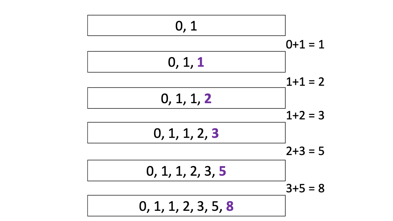
To calculate the Fibonacci number at position n, you store the first two numbers of the sequence, 0 and 1, in cache. Then, calculate the next numbers consecutively until you can return cache[n].

Generating the Fibonacci Sequence in Python

Now that you know the basics of how to generate the Fibonacci sequence, it’s time to go deeper and further explore the different ways to implement the underlying algorithm in Python. In the following sections, you’ll explore how to implement different algorithms to generate the Fibonacci sequence using recursion, Python object-oriented programming, and also iteration.

Using Recursion and a Python Class

Your first approach to generating the Fibonacci sequence will use a Python class and recursion. An advantage of using the class over the memoized recursive function you saw before is that a class keeps state and behavior (encapsulation) together within the same object. In the function example, however, cache is a completely separate object, so you don’t have control over it.

Below is the code that implements your class-based solution:

 1# fibonacci_class.py
 2
 3class Fibonacci:
 4    def __init__(self):
 5        self.cache = [0, 1]
 6
 7    def __call__(self, n):
 8        # Validate the value of n
 9        if not (isinstance(n, int) and n >= 0):
10            raise ValueError(f'Positive integer number expected, got "{n}"')
11
12        # Check for computed Fibonacci numbers
13        if n < len(self.cache):
14            return self.cache[n]
15        else:
16            # Compute and cache the requested Fibonacci number
17            fib_number = self(n - 1) + self(n - 2)
18            self.cache.append(fib_number)
19
20        return self.cache[n]

Here’s a breakdown of what’s happening in the code:

• Line 3 defines the Fibonacci class.
• Line 4 defines the class initializer, .__init__(). It’s a special method that you can use to initialize your class instances. Special methods are sometimes referred to as dunder methods, short for double underscore methods.
• Line 5 creates the .cache instance attribute, which means that whenever you create a Fibonacci object, there will be a cache for it. This attribute initially contains the first numbers in the Fibonacci sequence.
• Line 7 defines another special method, .__call__(). This method turns the instances of Fibonacci into callable objects.
• Lines 9 and 10 validate the value of n by using a conditional statement. If n is not a positive integer number, then the method raises a ValueError.
• Line 13 defines a conditional statement to check for those Fibonacci numbers that were already calculated and are available in .cache. If the number at index n is already in .cache, then line 14 returns it. Otherwise, line 17 computes the number, and line 18 appends it to .cache so you don’t have to compute it again.
• Line 20 returns the requested Fibonacci number.

To try this code, go ahead and save it into fibonacci_class.py. Then run this code in your interactive shell:>>>

>>> from fibonacci_class import Fibonacci

>>> fibonacci_of = Fibonacci()

>>> fibonacci_of(5)
5
>>> fibonacci_of(6)
8
>>> fibonacci_of(7)
13

>>> [fibonacci_of(n) for n in range(15)]
[0, 1, 1, 2, 3, 5, 8, 13, 21, 34, 55, 89, 144, 233, 377]

Here, you create and then call an instance of the Fibonacci class named fibonacci_of. The first call uses 5 as an argument and returns 5, which is the sixth Fibonacci number because you’re using zero-based indices.

This implementation of the Fibonacci sequence algorithm is quite efficient. Once you have an instance of the class, the .cache attribute holds the already computed numbers from call to call.

Visualizing the Memoized Fibonacci Sequence Algorithm

You can effectively understand how each call to a recursive Fibonacci function is handled using a call stack representation. The way each call is pushed onto the stack and popped off reflects exactly how the program runs. It clearly demonstrates how calculating large numbers will take a long time if you don’t optimize the algorithm.

In a call stack, whenever a function returns a result, a stack frame representing the function call is popped off the stack. Whenever you call a function, you add a new stack frame to the top of the stack. In general, this operation has a space complexity of O(n) because there are no more than n stack frames on the call stack at a single time.

Note: There’s a beginner-friendly code editor called Thonny that allows you to visualize the call stack of a recursive function in a graphical way. You can check out Thonny: The Beginner-Friendly Python Editor to learn more.

To visualize the memoized recursive Fibonacci algorithm, you’ll use a set of diagrams representing the call stack. The step number is indicated by the blue label below each call stack.

Say you want to compute F(5). To do this, you push the first call to the function onto the call stack:

To compute F(5), you must compute F(4) as outlined by the Fibonacci recurrence relation, so you add that new function call to the stack:

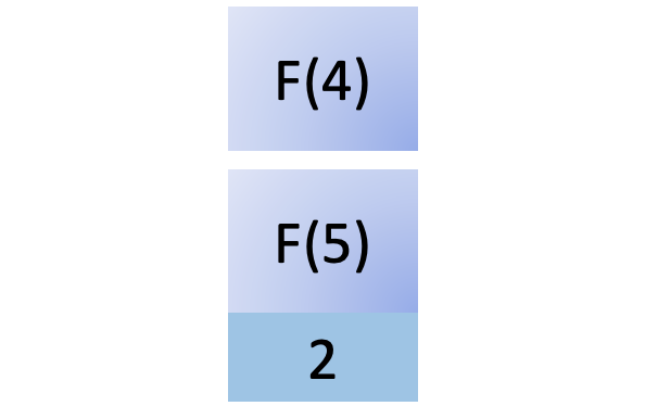
To compute F(4), you must compute F(3), so you add another function call to the stack:

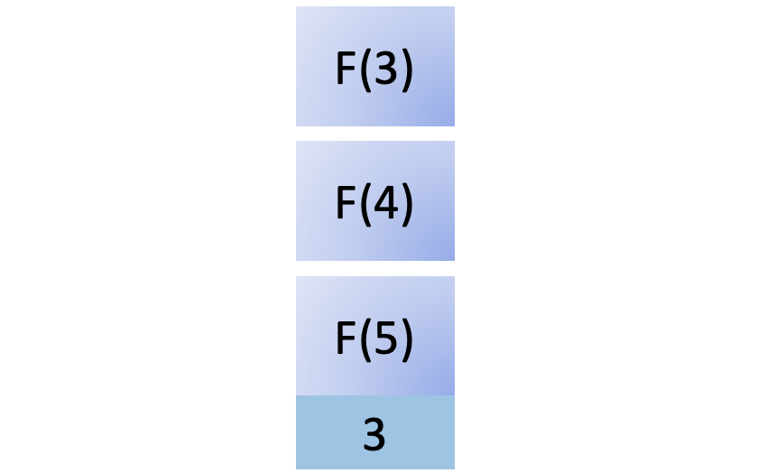
To compute F(3), you must compute F(2), so you add yet another function call to the call stack:

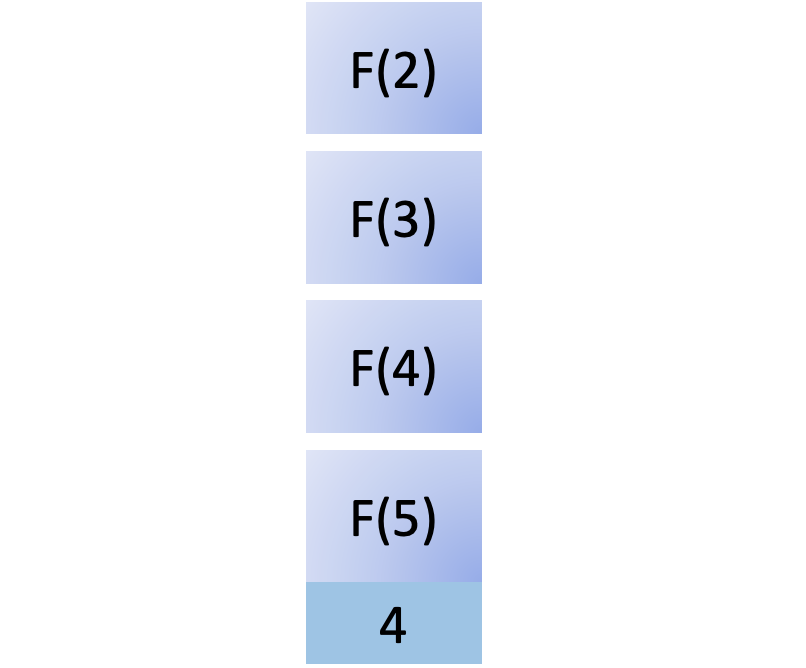
To compute F(2), you must compute F(1), so you add that to the stack. As F(1) is a base case, it returns immediately with 1, and you remove this call from the stack:

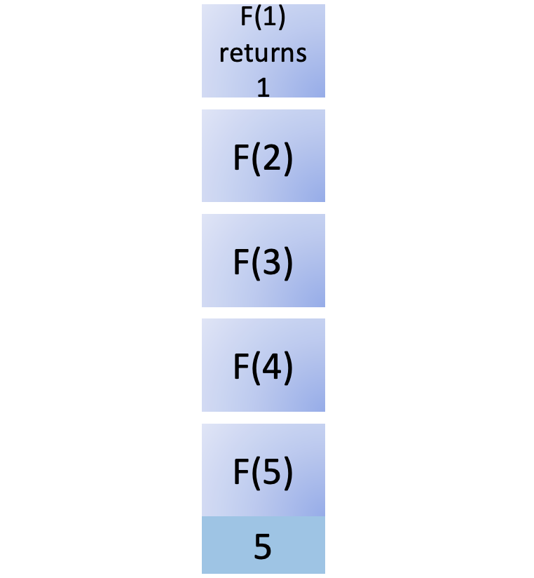
Now you start to unwind the results recursively. F(1) returns the result back to its calling function, F(2). To compute F(2), you also need to compute F(0):

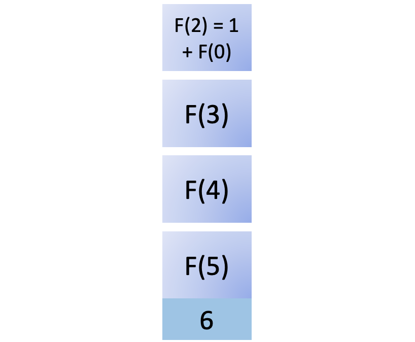
You add F(0) to the stack. Since F(0) is a base case, it returns immediately, giving you 0. Now you can remove it from the call stack:

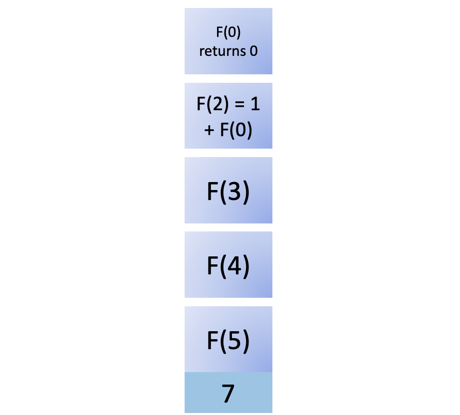
This result of calling F(0) is returned to F(2). Now you have what you need to compute F(2) and remove it from the stack:

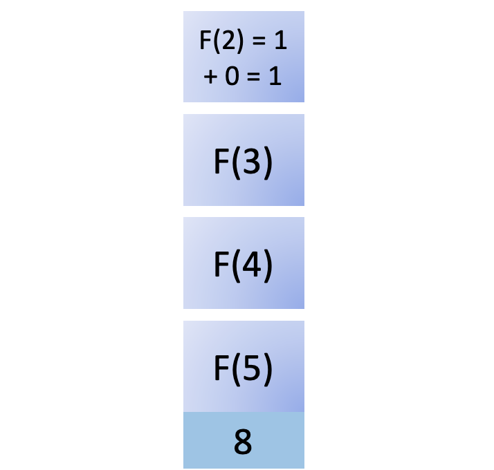
The result of F(2) is returned to its caller, F(3). F(3) also needs the results of F(1) to complete its calculation, so you add it back to the stack:

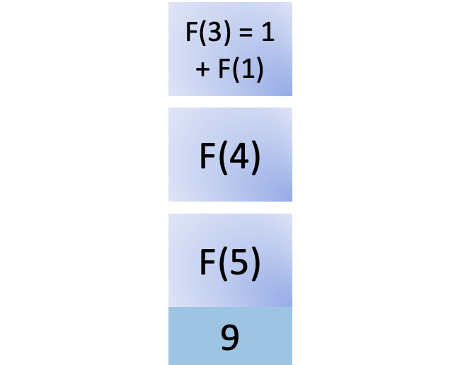
F(1) is a base case and its value is available in the cache, so you can return the result immediately and remove F(1) from the stack:

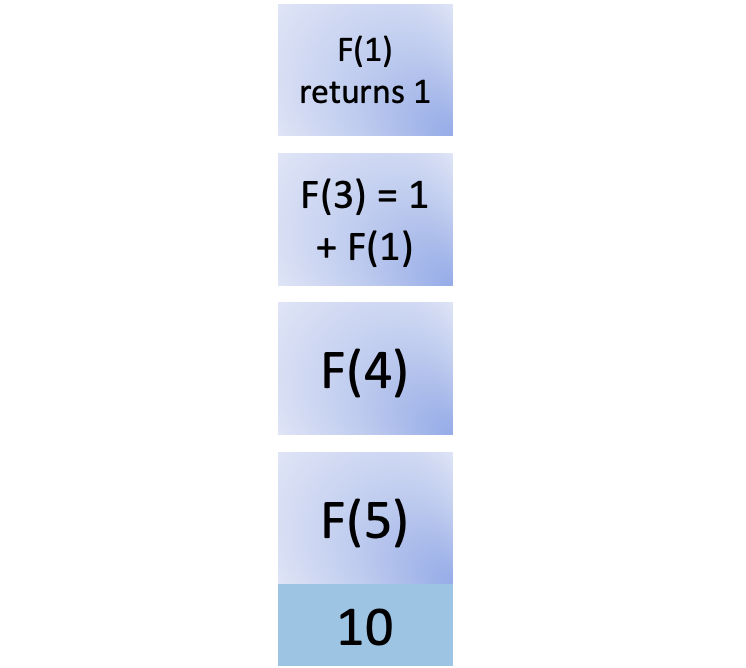
You can complete the calculation for F(3), which is 2:

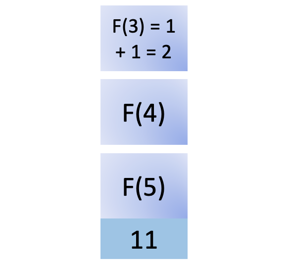
You remove F(3) from the stack after completing its calculation and return the result to its caller, F(4). F(4) also needs the result of F(2) to compute its value:

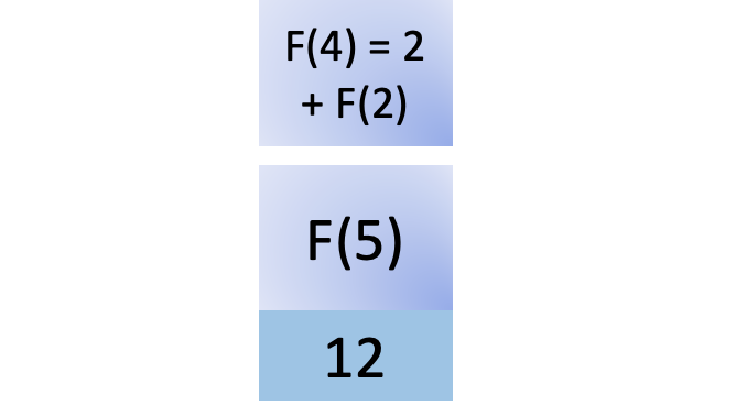
You push the call to F(2) onto the stack. This is where the nifty cache comes in. You have calculated it before, so you can just retrieve the value from the cache, avoiding a recursive call to compute the result of F(2) again. The cache returns 1, and you remove F(2) from the stack:

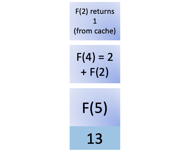
F(2) is returned to its caller, and now F(4) has all it needs to compute its value, which is 3:

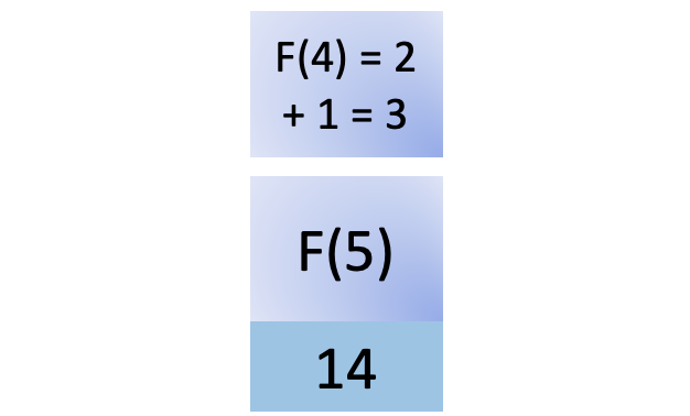
Next, you remove F(4) from the stack and return its result to the final and original caller, F(5):

F(5) now has the result of F(4) and also the result of F(3). You push an F(3) call onto the stack, and the nifty cache comes into play again. You previously calculated F(3), so all you need to do is retrieve it from the cache. There’s no recursive process to compute F(3). It returns 2, and you remove F(3) from the stack:

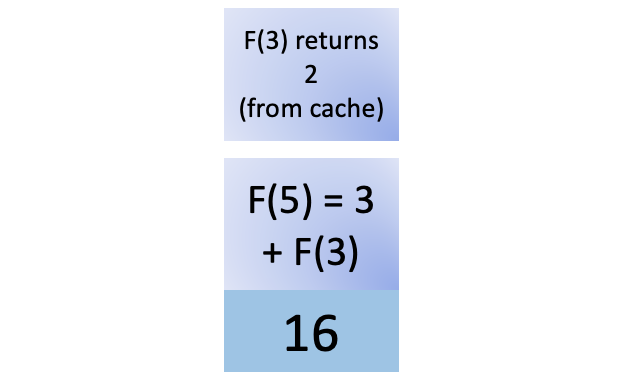
Now F(5) has all the values it needs to calculate its own value. You get 5 by adding 3 and 2, and that’s the final step before you pop the F(5) call off the stack. This action ends your sequence of recursive function calls:

The call stack is empty now. You’ve completed the final step to compute F(5):

Representing recursive function calls using a call stack diagram helps you understand all the work that takes place behind the scenes. It also allows you to see how many resources a recursive function can take up.

Putting all these diagrams together allows you to visualize how the whole process looks:

You can click the image above to zoom in on individual steps. If you don’t cache previously computed Fibonacci numbers, some of the stack stages in this diagram would be way taller, which means that they would take longer to return a result to their respective callers.

Using Iteration and a Python Function

The example in the previous sections implements a recursive solution that uses memoization as an optimization strategy. In this section, you’ll code a function that uses iteration. The code below implements an iterative version of your Fibonacci sequence algorithm:

 1# fibonacci_func.py
 2
 3def fibonacci_of(n):
 4    # Validate the value of n
 5    if not (isinstance(n, int) and n >= 0):
 6        raise ValueError(f'Positive integer number expected, got "{n}"')
 7
 8    previous, fib_number = 0, 1
 9    for _ in range(2, n + 1):
10        # Compute the next Fibonacci number, remember the previous one
11        previous, fib_number = fib_number, previous + fib_number
12
13    return fib_number

Now, instead of using recursion in fibonacci_of(), you’re using iteration. This implementation of the Fibonacci sequence algorithm runs in O(n) linear time. Here’s a breakdown of the code:

• Line 3 defines fibonacci_of(), which takes a positive integer, n, as an argument.
• Lines 5 and 6 perform the usual validation of n.
• Line 8 defines two local variables, previous and fib_number, and initializes them with the first two numbers in the Fibonacci sequence.
• Line 9 starts a for loop that iterates from 2 to n + 1. The loop uses an underscore (_) for the loop variable because it’s a throwaway variable and you won’t be using this value in the code.
• Line 11 computes the next Fibonacci number in the sequence and remembers the previous one.
• Line 13 returns the requested Fibonacci number.

To give this code a try, get back to your interactive session and run the following code:>>>

>>> from fibonacci_func import fibonacci_of

>>> fibonacci_of(5)
5
>>> fibonacci_of(6)
8
>>> fibonacci_of(7)
13

>>> [fibonacci_of(n) for n in range(15)]
[0, 1, 1, 2, 3, 5, 8, 13, 21, 34, 55, 89, 144, 233, 377]

This implementation of fibonacci_of() is quite minimal. It uses iterable unpacking to compute the Fibonacci numbers during the loops, which is quite efficient memory-wise. However, every time you call the function with a different value of n, it has to recompute the sequence over again. To fix this, you can use closures and make your function remember the already computed values between calls. Go ahead and give it a try!

Conclusion

The Fibonacci sequence can help you improve your understanding of recursion. In this tutorial, you’ve learned what the Fibonacci sequence is. You’ve also learned about some common algorithms to generate the sequence and how to translate them into Python code.

The Fibonacci sequence can be an excellent springboard and entry point into the world of recursion, which is a fundamental skill to have as a programmer.

In this tutorial, you learned how to:

• Generate the Fibonacci sequence using a recursive algorithm
• Optimize your recursive Fibonacci algorithm using memoization
• Generate the Fibonacci sequence using an iterative algorithm

You’ve also visualized the memoized recursive algorithm to get a better understanding of how it works behind the scenes. To do that, you used a call stack diagram.

Once you master the concepts in this tutorial, your Python programming skills will improve along with your recursive algorithmic thinking.